A Replicable Method for Gathering, Analysing and Visualising Podcast Episode and Review Data - Part 1
Rate and Review - Part 1
I’m currently writing a journal article with a colleague, and the research behind it has involved the collection and analysis of data related to music podcasts. During the course of undertaking this work, I have developed a workflow able to gather data for ~9,000 podcast episodes and ~18,000 reviews from the input of a single URL. This post presents that process as a replicable workflow.
I hope you find the process useful. Please do let me know if you use it. I would be very interested to see what kind of results are produced if this method was applied to different genres of podcast.
Please feel free to drop me a line if you have any questions about it, or if you would like to discuss ways we can work together.
Overview
This post and the others following in the mini-series will provide a workthrough for researchers interested in gathering and analysing data about podcasts. The workflow consists of four parts:
- Part 1: gathers episode and review data for a given set of podcasts.
- Part 2: prepares that data and then runs a handful of NLP analyses
- Part 3: visualises and explores the of results.
- Part 4: creates an interactive web document allowing users to explore results.
Part 1 takes as its starting point the URL of given podcast chart published on the Chartable website. From there, information about podcast episodes and reviews submitted to the Apple podcast store is automatically collected. Part 2 walks through some data tidying, before then analysing the text contained within reviews using NLP algorthims, to help reveal broad ‘themes’ across a corpus of reviews and to also analyse sentiment. In Part 3, the data collected and the results of the NLP analyses are combined and visualised, before finally - in Part 4 - the results are published as an interactive web document.
Prerequisties
Before attempting to run the code contained within this post you will need the following:
- The latest installation of R - visit The R Project website for more information and download links.
- R Studio - visit the R Studio website for more information and download links.
- An account on ShinyApps.io - this is where you will eventually host the interactive webpage you create in Part 4.
R and R Studio are available as free, open source downloads and there are a huge number of resources online that will help you get started. The links above will explain those resources and the installation processes. An account on ShinyApps.io is also available for free, but access to your page will be subject to a monthly usage cap. For more information on hosting Shiny documents, see this guide.
The workflow contained in the series assumes a degree of confidence/profficiency with the R language. At certain stages of the process, you will be required to make decisions on which data to include or remove, which will require amending the code I have supplied. That being said, the workflow has also been designed to act as a tutorial of sorts. Researchers new to R should be able to copy the code provided into their own workspace and follow through the process.
1: Load Packages
To begin, you will need to load the following R packages:
#If not previously installed, run:
#install.packages('name of package')
library(rvest)
library(tidyverse)
library(DT)
library(itunesr)
2: Get Chartable Data
The starting point for gathering episode and review data is the Chartable website.
Chartable is a data analytics service that gathers metrics associated with podcasts. It is used primarily by podcast producers as a means of understanding the size, reach and composition of their audiences, and by advertisers seeking to understand the effectiveness of ads reaching those podcast audiences. Chartable offers a paid tier service that provides access to numerous metrics and analytical tools.
On Chartable’s publicly-accessibly site, however, they also provide information on podcast charts published by numerous services, broken down into numerous genres and sub-genres. Charts and/or the performance of a particular podcast can be viewed at the Chartable Charts page.
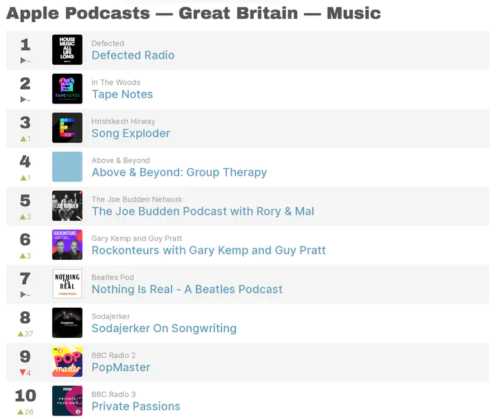
One collection of charts available from the Chartable service is the Apple Podcast Charts. The chart analysed in this workflow is the Apple Podcasts - Great Britain - Music chart, using data gathered on 6th April 2021.
As Apple Podcast charts are updated regularly, a snapshot of the chart being analysed was archived by the research team using the WayBackMachine internet archive. The Chartable page containing chart data as it appeared on 6th April 2021 can be viewed here. A screenshot of the page is provided below.
 The first step in the data gathering process is to extract the names and chart positions of podcasts in a given chart.
To do this, you will need to create the get_podcast_chart function below. This function uses the rvest package to extract information from a given URL. The data is then organised into a dataframe called podcast_info.
# Create Function

get_podcast_chart <- function(chart_url, name) {
  webpage <- read_html(chart_url)
  podcast_names <- html_nodes(webpage,'.f3 a')
  podcast_info <- as.data.frame(html_text(podcast_names))
  podcast_info$chartable_url <- as.data.frame(html_attr(podcast_names, 'href'))
  podcast_info <- podcast_info[3:nrow(podcast_info), ]
  podcast_info$chart_position <- 1:nrow(podcast_info)
  podcast_info$chart <- chart_name
  podcast_info$date <- Sys.Date()
  podcast_info <- podcast_info[, c(3:5, 1:2)]
  podcast_info <- podcast_info %>%
    rename(podcast = `html_text(podcast_names)`)
  podcast_info$chartable_url$`html_attr(podcast_names, "href")`
  urls <- podcast_info$chartable_url$`html_attr(podcast_names, "href")`
  podcast_info$chartable_url <- urls
  rm(webpage, podcast_names, urls)
  #write_rds(podcast_info, "podcast_chart_info.rds") - if you want to write out the result as an RDS file
  return(podcast_info)
}
You can use the function get_podcast_chart to fetch information for the chart of your choice by creating two new objects:
- chart_url - the full URL of the Chartable page you want to scrape
- chart_name - the name of the chart you are scraping data for
Once these objects are created, you can pass them to the get_podcast_chart function and assign the result to podcast_info.
chart_url <- 'https://chartable.com/charts/itunes/gb-music-podcasts'
chart_name <- "Apple Podcasts - Great Britain - Music"
podcast_info <- get_podcast_chart(chart_url, chart_name)
The resulting podcast_info dataframe will contain 5 variables:
- chart_postion - the position of a podcast in the Chartable chart
- chart - the name of the chart
- date - the date the information was retrieved
- podcast - the name of the podcast
- chartable_url - the individual URL for a podcast’s page on Chartable’s site.
The final variable here - chartable_url - is important because it is on the individual podcast pages where you will find the links to both the RSS feed for a given podcast and the URL for that podcast on Apple’s store. It is this information that will enable the collection of episode and reviews data.
str(podcast_info)## 'data.frame': 100 obs. of 5 variables:
## $ chart_position: int 1 2 3 4 5 6 7 8 9 10 ...
## $ chart : chr "Apple Podcasts - Great Britain - Music" "Apple Podcasts - Great Britain - Music" "Apple Podcasts - Great Britain - Music" "Apple Podcasts - Great Britain - Music" ...
## $ date : Date, format: "2021-04-06" "2021-04-06" ...
## $ podcast : chr "Defected Radio" "Tape Notes" "Song Exploder" "Above & Beyond: Group Therapy" ...
## $ chartable_url : chr "https://chartable.com/podcasts/defected-radio" "https://chartable.com/podcasts/tape-notes" "https://chartable.com/podcasts/song-exploder" "https://chartable.com/podcasts/above-beyond-group-therapy" ...IMPORTANT
So far, this process will have collected data on 100 podcasts - which is the number displayed on Chartable’s site for a given Apple podcast chart. If you want to work through this workflow to test out how it works, you may wish to reduce the number of podcasts you are collecting data for. Collecting data for 100 podcasts takes approximately 2 hours. If you reduce the field of podcasts to the first three shows in the chart using the code below, the process will run through much more quickly.
The rest of this workflow shows examples and data from our process, which involved collecting and analysing data on the top 50 shows in the music chart. Your results for 3 podcasts will appear in the same way.
podcast_info <- podcast_info[1:3,] ##to select instead the first ten podcasts, amend 1:3 to 1:10. And so on. Once you have selected how many of the podcasts in a given chart you wish to analyse, you can proceed to the next section.
3: Extract RSS and Apple IDs
On each individual Chartable page for given podcast, you will find the RSS feed and the URL for that podcast on the Apple store. In the screenshot below, the Chartable page for the podcast ranked #1 in the chart on the date analysed is shown.
The next stage of the process is to extact that RSS feed and Apple store page link information from each podcast page.

The code below extracts the information circled in the image above for the first podcast in the podcast_info dataframe and writes this to a new dataframe, links.
url <- podcast_info$chartable_url[[1]]
podcast <- podcast_info$podcast[[1]]
webpage <- read_html(url)
podcast_page <- html_nodes(webpage,'.f6 a')
podcast_links <- as.data.frame(html_text(podcast_page))
podcast_links$urls <- as.data.frame(html_attr(podcast_page, 'href'))
rss_apple <- podcast_links %>%
  filter(`html_text(podcast_page)` == "RSS feed" | `html_text(podcast_page)` == "Listen on Apple Podcasts")
links <- as.data.frame(podcast)
links$chartable_url <- url
rss_apple <- as.data.frame(rss_apple$url)
links$rss <- rss_apple$`html_attr(podcast_page, "href")`[[1]]
links$apple <- rss_apple$`html_attr(podcast_page, "href")`[[2]]
links$apple_id <- gsub(".*id", "", links$apple[[1]])
links$apple_id <- sub("at.*", "", links$apple_id)
links$apple_id <- str_remove(links$apple_id, "[?]")
links$apple_id <- as.numeric(links$apple_id)
As you can see below, for the podcast in question we now have the following information:
- podcast - the name of the podcast.
- chartable_url - the podcast page on Chartable.
- rss - the RSS feed address for the podcast (from where we’ll get episode data).
- apple - the URL for the podcast on Apple’s store (containing the Apple ID for the podcast).
- apple_id - the unique Apple ID extracted from the apple variable (with which we can get reviews and ratings data).
str(links)## 'data.frame': 1 obs. of 5 variables:
## $ chartable_url : chr "https://chartable.com/podcasts/defected-radio"
## $ chart_position: int 1
## $ rss : chr "https://portal-api.thisisdistorted.com/xml/defected-in-the-house"
## $ apple : chr "https://itunes.apple.com/us/podcast/id120107389?at=1001lMGa&ct=podcast%3ADJMxkvn6"
## $ apple_id : num 1.2e+08Having extracted this information for one podcast, we can do the same for the others in the podcast_info dataframe.
NB: The code below contains a number of messages that will appear in your console to give you an indication of progress.
for (i in 2:nrow(podcast_info)) {
  url <- podcast_info$chartable_url[[i]]
  podcast <- podcast_info$podcast[[i]]
  number <- podcast_info$chart_position[[i]]
  print(paste("Getting info for", podcast, ": Number", number, sep = " "))
  webpage <- read_html(url)
  podcast_page <- html_nodes(webpage,'.f6 a')
  podcast_links <- as.data.frame(html_text(podcast_page))
  podcast_links$url <- as.data.frame(html_attr(podcast_page, 'href'))
  rss_apple <- podcast_links %>%
    filter(`html_text(podcast_page)` == "RSS feed" | `html_text(podcast_page)` == "Listen on Apple Podcasts")
  links_new <- as.data.frame(podcast)
  links_new$chartable_url <- url
  rss_apple <- as.data.frame(rss_apple$url)
  links_new$rss <- rss_apple$`html_attr(podcast_page, "href")`[[1]]
  links_new$apple <- rss_apple$`html_attr(podcast_page, "href")`[[2]]
  links_new$apple_id <- gsub(".*id", "", links_new$apple[[1]])
  links_new$apple_id <- sub("at.*", "", links_new$apple_id)
  links_new$apple_id <- str_remove(links_new$apple_id, "[?]")
  links_new$apple_id <- as.numeric(links_new$apple_id)
  links <- rbind(links, links_new)
  rm(links_new, rss_apple, podcast_links)
  print(paste("Waiting", 5, "seconds before getting next podcast", sep = " "))
  Sys.sleep(5)
}
Once this process is completed, you can then merge the podcast_info dataframe with the links dataframe using the common chartable_url variable, creating a new dataframe, podcast_links.
podcast_links <- merge(podcast_info,links, by="chartable_url")
podcast_links <- podcast_links[order(podcast_links$chart_position),]
podcast_links$podcast.x <- NULL
podcast_links <- podcast_links %>%
  rename(podcast = podcast.y)
rm(links, podcast_info, podcast_page, webpage, i, number, podcast, url, chart_name, chart_url, get_podcast_chart)
The resulting podcast_links data frame contains 8 variables.
NB: In the example below, information for 100 podcasts is contained. If you decided to reduce the number of podcasts in step 2, you will have the number of podcasts you reduced down to.
- chartable_url - the podcast page on Chartable
- chartable_position - the position in the podcast chart
- chart - the name of the podcast chart
- date - the date the chart information was captured
- podcast - the name of the podcast
- rss - the RSS feed address for the podcast
- apple - the URL for the podcast on Apple’s store
- apple_id - the unique Apple ID extracted apple
str(podcast_links)## 'data.frame': 100 obs. of 8 variables:
## $ chartable_url : chr "https://chartable.com/podcasts/defected-radio" "https://chartable.com/podcasts/tape-notes" "https://chartable.com/podcasts/song-exploder" "https://chartable.com/podcasts/above-beyond-group-therapy" ...
## $ chart_position: int 1 2 3 4 5 6 7 8 9 10 ...
## $ chart : chr "Apple Podcasts - Great Britain - Music" "Apple Podcasts - Great Britain - Music" "Apple Podcasts - Great Britain - Music" "Apple Podcasts - Great Britain - Music" ...
## $ date : Date, format: "2021-04-06" "2021-04-06" ...
## $ podcast : chr "Defected Radio" "Tape Notes" "Song Exploder" "Above & Beyond: Group Therapy" ...
## $ rss : chr "https://portal-api.thisisdistorted.com/xml/defected-in-the-house" "https://tapenotes.libsyn.com/rss" "http://feed.songexploder.net/SongExploder" "http://static.aboveandbeyond.nu/grouptherapy/podcast.xml" ...
## $ apple : chr "https://itunes.apple.com/us/podcast/id120107389?at=1001lMGa&ct=podcast%3ADJMxkvn6" "https://itunes.apple.com/us/podcast/id1249834293?at=1001lMGa&ct=podcast%3AX6XZXD0W" "https://itunes.apple.com/us/podcast/id788236947?at=1001lMGa&ct=podcast%3A369dyG5E" "https://itunes.apple.com/us/podcast/id286889904?at=1001lMGa&ct=podcast%3A0E4lVDYE" ...
## $ apple_id : num 1.20e+08 1.25e+09 7.88e+08 2.87e+08 1.54e+09 ...The podcast_links dataframe now contains all the information we require to extract episode and reviews data.
For the purposes of the article this script was written for, we wanted to concentrate on only the Top 50 podcasts in the chart. Before proceeding to the next section, we can remove those podcasts in places lower than 50. This is a similar process to that described in step 2 above.
We can see that
podcast_links begins with 100 rows. By filtering this for chart positions lower than 51, we reduce the number of rows to 50.
nrow(podcast_links)## [1] 100podcast_links <- podcast_links %>%
filter(chart_position < 51)
nrow(podcast_links)## [1] 504: Get Episode Data
Using the rss element of the podcast_links dataframe created in the steps above, we can now extract episode data for each podcast.
For an explanation of how RSS feeds and podcasts work together, see this article
The RSS feed for a given podcast will contain information for every episode delivered and each RSS feed will follow the same/similar format, with information organised according to a number of common variables. In the image below, we can see that the description of each podcast episode is heled within the itunes:summary element, the episode length is in itunes:duration, and the publication date is within pubDate.
This information is replicated for each episode of a given podcast within it’s RSS feed, and the RSS feeds for other podcasts will follow the same format. Based on this, and assuming the RSS feed address we have collected is correct, we can extract episode information for each podcast.

To demonstrate this, the code below extracts information from the RSS feed for the first podcast in the podcast_links dataframe and writes it to new dataframe, episode_data.
Note in the code that elements displayed in the image above are present. Elements such as pubDate and itunes:summary become varialbes within the episode_data dataframe.
podcast_name <- podcast_links$podcast[[1]]
rss <- podcast_links$rss[[1]]
pod_id <- podcast_links$apple_id[[1]]
chart <- podcast_links$chart[[1]]
chart_week <- podcast_links$date[[1]]
chart_position <- podcast_links$chart_position[[1]]
css_descriptors <- c('title', 'pubDate', 'itunes\\:summary', 'itunes\\:duration') # XML tags of interest
col_names <- c('title', 'pubdate','summary', 'duration') # Initial column names for tibble
# Load XML feed and extract items nodes
podcast_feed <- read_xml(rss)
items <- xml_nodes(podcast_feed, 'item')
# Extracts from an item node the content defined by the css_descriptor
extract_element <- function(item, css_descriptor) {
  element <- xml_node(item, css_descriptor) %>% xml_text
  element
}
episode_data <- sapply(css_descriptors, function(x) {
  extract_element(items, x)}
) %>% as_tibble()
names(episode_data) <- col_names # Set new column names
episode_data$podcast <- podcast_name
episode_data$rss <- rss
episode_data$pod_id <- pod_id
episode_data$chart <- chart
episode_data$chart_week <- chart_week
episode_data$chart_position <- chart_position
episode_data$episode_id <- nrow(episode_data):1
episode_data <- episode_data[c(5:11, 1:4)]
Running the code above produces the episode_data dataframe, which contains the following variables:
- podcast - the name of the podcast.
- rss - the rss feed of the podcast.
- pod_id - the apple id.
- chart - the chart from which this data came.
- chart_week - the date the data was retrieved.
- chart_position -the position of the podcast in that chart.
- episode_id - the episode number.
- title - the episode title.
- pubdate - the date the episode was released.
- summary - the episode summary.
- duration - the duration of the episode.
str(episode_data)## tibble [1 × 11] (S3: tbl_df/tbl/data.frame)
## $ podcast : chr "Defected Radio"
## $ rss : chr "https://portal-api.thisisdistorted.com/xml/defected-in-the-house"
## $ pod_id : num 1.2e+08
## $ chart : chr "Apple Podcasts - Great Britain - Music"
## $ chart_week : Date[1:1], format: "2021-04-06"
## $ chart_position: int 1
## $ episode_id : int 450
## $ title : chr "Defected Radio Show: Masters At Work Takeover - 02.04.21"
## $ pubdate : chr "Fri, 02 Apr 2021 08:00:00 +0000"
## $ summary : chr "\nPodcast from Defected Records \n <br /><br />LOUIE VEGA (Hour 1)<br />\t1\tDJ Spen Feat. Fo"| __truncated__
## $ duration : chr "02:04:50"Having obtained the episode data from the first show in the podcast_links dataframe, and because the data contained within the RSS feeds for all podcasts in the list is common, the code below loops through the remaining shows in the dataframe in order to extract further episode information.
for (i in 2:nrow(podcast_links)) {
  try ({
    episode_data <- episode_data
    podcast_name <- podcast_links$podcast[[i]]
    print(paste("Getting info for", podcast_name, sep = " "))
    rss <- podcast_links$rss[[i]]
    pod_id <- podcast_links$apple_id[[i]]
    chart <- podcast_links$chart[[i]]
    chart_week <- podcast_links$date[[i]]
    chart_position <- podcast_links$chart_position[[i]]
    css_descriptors <- c('title', 'pubDate', 'itunes\\:summary', 'itunes\\:duration') # XML tags of interest
    col_names <- c('title', 'pubdate','summary', 'duration') # Initial column names for tibble
    # Load XML feed and extract items nodes
    podcast_feed <- read_xml(rss)
    items <- xml_nodes(podcast_feed, 'item')
    # Extracts from an item node the content defined by the css_descriptor
    extract_element <- function(item, css_descriptor) {
      element <- xml_node(item, css_descriptor) %>% xml_text
      element
    }
    episodes <- sapply(css_descriptors, function(x) {
      extract_element(items, x)}
    ) %>% as_tibble()
    names(episodes) <- col_names # Set new column names
    episodes$podcast <- podcast_name
    episodes$rss <- rss
    episodes$pod_id <- pod_id
    episodes$chart <- chart
    episodes$chart_week <- chart_week
    episodes$chart_position <- chart_position
    episodes$episode_id <- nrow(episodes):1
    episodes <- episodes[c(5:11, 1:4)]
    episode_data <- rbind(episode_data, episodes)
    rm(episodes)
  })
}
The final results will be contained in the episode_data dataframe.
Before moving on, we can check to see if any podcasts are missing from the list. Remember that we filtered the original podcast_links file to contain only the top 50 podcasts. Ideally, the number of podcasts_missing will be zero, and there will be 50 unique pod_ids in episode_data. This appears to be the case!
episode_data_ids <- unique(episode_data$pod_id)
podcasts_missing <- podcast_links %>%
  filter(!apple_id %in% episode_data_ids)
nrow(podcasts_missing)
## [1] 0length(unique(episode_data$pod_id))## [1] 50At this stage you can remove some elements from your R enviroment.
rm(items, podcast_feed, chart, chart_position,
   chart_week, col_names, css_descriptors, episode_data_ids, i, pod_id, podcast_name, rss, extract_element, podcasts_missing)
5 Get Reviews Data
As with extracting episode data above, finding review data uses an element of podcast_links. This time, the apple_id is used with the itunesr package.
The getReviews function takes three arguements.
- the first is the unique Apple ID of a podcast (which we have in the apple_id variable)
- the second is a unique country code of the Apple store in which a review was posted - there are 155 national Apple stores (more on this in a moment)
- the third argument is a page number. Podcast reviews in national Apple stores are organised into pages (again, more on this in a moment).
To demonstrate this function, we can retrieve the 1st page of reviews from the GB (Great Britain) store for the first podcast in our list.
Here, the arguments passed to getReviews are: the first apple_id in podcast_links; the text string ‘gb’; and the number 1.
pod_id <- podcast_links$apple_id[[1]]
#Create reviews template
page <- 1
reviews <- getReviews(pod_id,'gb', page) #needs ID, country and page #
reviews$country <- 'gb'
reviews$podcast <- podcast_links$podcast[[1]]
reviews$pod_id <- podcast_links$apple_id[[1]]
reviews$review_page <- page
reviews <- reviews[, c(9:11, 1:8)]
We can see from the results that the first podcast in our list has 49 reviews in the GB store.
Apple organises reviews by page for a given country store, and 49 is the maximum number of reviews that appear on a page. Because we have retrieved 49 reviews on page 1, we can assume that there is a second page of reviews we can retrieve.
We also know that there are other national Apple stores which may also contain reviews, and possibly several pages of reviews in each of those.
str(reviews)## 'data.frame': 49 obs. of 11 variables:
## $ podcast : chr "Defected Radio" "Defected Radio" "Defected Radio" "Defected Radio" ...
## $ pod_id : num 1.2e+08 1.2e+08 1.2e+08 1.2e+08 1.2e+08 ...
## $ review_page: num 1 1 1 1 1 1 1 1 1 1 ...
## $ Title : chr "Love this show!" "Awesome show." "Keep on running 🏃♂️" "Great podcast" ...
## $ Author_URL : chr "https://itunes.apple.com/gb/reviews/id652281798" "https://itunes.apple.com/gb/reviews/id31107582" "https://itunes.apple.com/gb/reviews/id24598886" "https://itunes.apple.com/gb/reviews/id588974749" ...
## $ Author_Name: chr "Toots Fontaine" "barclayreviews" "strab1964" "Gareth870" ...
## $ App_Version: chr "" "" "" "" ...
## $ Rating : chr "5" "5" "5" "5" ...
## $ Review : chr "Been listening to this for a few years now and you’re a life saver. Keep on keeping on xx" "Track list please?" "From my first ever introduction to Defected House in Ibiza , I was hooked ! And now is the soundtrack to my mor"| __truncated__ "Love the weekly defected podcasts especially the glitterbox sessions showcasing proper disco music. Only critic"| __truncated__ ...
## $ Date : POSIXct, format: "2021-03-18 11:38:27" "2021-02-20 07:02:52" ...
## $ country : chr "gb" "gb" "gb" "gb" ...In order to gather data from non-GB stores, we first need to create a list of global Apple stores. The code below will create a dataframe called apple containing unique country codes for 155 national Apple stores, along with another variable containing the country name.
code <- c("al", "dz", "ao", "ai", "ag", "ar", "am", "au", "at", "az",
          "bs", "bh", "bb", "by", "be", "bz", "bj", "bm", "bt", "bo",
          "bw", "br", "vg", "bn", "bg", "bf", "kh", "ca", "cv", "ky",
          "td", "cl", "cn", "co", "cr", "hr", "cy", "cz", "cg", "dk",
          "dm", "do", "ec", "eg", "sv", "ee", "fm", "fj", "fi", "fr",
          "gm", "de", "gh", "gb", "gr", "gd", "gt", "gw", "gy", "hn",
          "hk", "hu", "is", "in", "id", "ie", "il", "it", "jm", "jp",
          "jo", "kz", "ke", "kg", "kw", "la", "lv", "lb", "lr", "lt",
          "lu", "mo", "mk", "mg", "mw", "my", "ml", "mt", "mr", "mu",
          "mx", "md", "mn", "ms", "mz", "na", "np", "nl", "nz", "ni",
          "ne", "ng", "no", "om", "pk", "pw", "pa", "pg", "py", "pe",
          "ph", "pl", "pt", "qa", "tt", "ro", "ru", "kn", "lc", "vc",
          "st", "sa", "sn", "sc", "sl", "sg", "sk", "si", "sb", "za",
          "kr", "es", "lk", "sr", "sz", "se", "ch", "tw", "tj", "tz",
          "th", "tn", "tr", "tm", "tc", "ug", "ua", "ae", "us", "uy",
          "uz", "ve", "vn", "ye", "zw")

country <- c("Albania", "Algeria", "Angola", "Anguilla", "Antigua and Barbuda",
             "Argentina", "Armenia", "Australia", "Austria", "Azerbaijan", "Bahamas",
             "Bahrain", "Barbados", "Belarus", "Belgium", "Belize", "Benin", "Bermuda",
             "Bhutan", "Bolivia", "Botswana", "Brazil", "British Virgin Islands",
             "Brunei Darussalam", "Bulgaria", "Burkina-Faso", "Cambodia", "Canada",
             "Cape Verde", "Cayman Islands", "Chad", "Chile", "China", "Colombia",
             "Costa Rica", "Croatia", "Cyprus", "Czech Republic",
             "Democratic Republic of the Congo", "Denmark", "Dominica", "Dominican Republic",
             "Ecuador", "Egypt", "El Salvador", "Estonia", "Federated States of Micronesia",
             "Fiji", "Finland", "France", "Gambia", "Germany", "Ghana", "Great Britain",
             "Greece", "Grenada", "Guatemala", "Guinea Bissau", "Guyana", "Honduras",
             "Hong Kong", "Hungaria", "Iceland", "India", "Indonesia", "Ireland",
             "Israel", "Italy", "Jamaica", "Japan", "Jordan", "Kazakhstan",
             "Kenya", "Krygyzstan", "Kuwait", "Laos", "Latvia", "Lebanon",
             "Liberia", "Lithuania", "Luxembourg", "Macau", "Macedonia",
             "Madagascar", "Malawi", "Malaysia", "Mali", "Malta", "Mauritania",
             "Mauritius", "Mexico", "Moldova", "Mongolia", "Montserrat", "Mozambique",
             "Namibia", "Nepal", "Netherlands", "New Zealand", "Nicaragua", "Niger",
             "Nigeria", "Norway", "Oman", "Pakistan", "Palau", "Panama",
             "Papua New Guinea", "Paraguay", "Peru", "Philippines", "Poland",
             "Portugal", "Qatar", "Republic of Trinidad and Tobago", "Romania",
             "Russia", "Saint Kitts and Nevis", "Saint Lucia",
             "Saint Vincent and the Grenadines", "Sao Tome e Principe",
             "Saudi Arabia", "Senegal", "Seychelles", "Sierra Leone",
             "Singapore", "Slovakia", "Slovenia", "Soloman Islands",
             "South Africa", "South Korea", "Spain", "Sri Lanka",
             "Suriname", "Swaziland", "Sweden", "Switzerland",
             "Taiwan", "Tajikistan", "Tanzania", "Thailand", "Tunisia",
             "Turkey", "Turkmenistan", "Turks and Caicos Islands",
             "Uganda", "Ukraine", "United Arab Emirates",
             "United States of America", "Uruguay", "Uzbekistan",
             "Venezuela", "Vietnam", "Yemen", "Zimbabwe")

apple <- as.data.frame(cbind(code, country))
str(apple)
## 'data.frame': 155 obs. of 2 variables:
## $ code : chr "al" "dz" "ao" "ai" ...
## $ country: chr "Albania" "Algeria" "Angola" "Anguilla" ...Based on the above, the code below loops through each of the 155 Apple store codes and checks for reviews for the first podcast in our list.
If no reviews are found for a particular national store, the script moves on the next store.
If 49 reviews are found on the first page for a particular country, the script will then check for reviews on page 2. If 49 reviews are found on page 2, the script will check page 3. And so on, until a page is returned with fewer than 49 reviews. If the nth page contains fewer than 49 reviews, the script then moves on to the next country store.
Once the process completes, the script removes the duplicated entries (for page 1, GB store) collected in the earlier demonstration step.
IMPORTANT: A key limitation of this method is that Apple appear to block the getReviews function if the page number is greater than 10. I’m not sure why this is, and I could not produce a workaround. Instead, the script has a mechanism to move on to another national store once the page number being checked reaches 10. This will will of course restrict your results to 490 national reviews for a given podcast (49 per page, times 10 pages), but for the vast majority of podcasts/countries, this figure will likely be sufficient. Indeed, it may only be a problem if the podcast in question is exceptionally popular in a particular national market, and/or that national market is large. In the case of the 50 podcasts studied by this research, 10 podcasts reached this limit either in the US and GB stores. Clearly, this means that any analysis of reviews data must take into account the timeframe covered by the incomplete reviews.
pod_id <- podcast_links$apple_id[[1]]
podcast <- podcast_links$podcast[[1]]

for (i in 1:nrow(apple)) {
  try({
    page = 1
    x <- apple$code[[i]]
    y <- apple$country[[i]]
    print(paste("Now looking at", y, "for", podcast, sep = " "))
    reviews_test <- getReviews(pod_id, x, page)
    reviews_test$country <- x
    reviews_test$podcast <- podcast
    reviews_test$pod_id <- pod_id
    reviews_test$review_page <- page
    reviews_test <- reviews_test[, c(9:11, 1:8)]
    reviews <- rbind(reviews, reviews_test)
    if (nrow(reviews_test) == 49)
      repeat {
        try({
          rm(reviews_test)
          wait_time <- sample(10:20, 1)
          print(paste("Waiting", wait_time, "seconds before checking page", page + 1, "for", y, "for", podcast, sep = " "))
          Sys.sleep(wait_time)
          page = page + 1
          if (page > 10) break
          reviews_test <- getReviews(pod_id, x , page)
          reviews_test$country <- x
          reviews_test$podcast <- podcast
          reviews_test$pod_id <- pod_id
          reviews_test$review_page <- page
          reviews_test <- reviews_test[, c(9:11, 1:8)]
          reviews <- rbind(reviews, reviews_test)
          if (nrow(reviews_test) < 49) break
        })#, silent = T)
      }
  }, silent = T)
}

reviews <- reviews[!duplicated(reviews$Review), ]
Having gathered reviews for the first podcasts for each country store, this next part of the script repeats the process above for the rest of the podcasts. It contains a number of text updates and that will show you the progress as it iterates through each podcast, each country, and up to 10 pages of reviews.
NB: Gathering reviews data for 50 podcasts in the Apple Music Chart took around 2 hours. If you are collecting a similar number, you may wish to ensure your machine remains connected to the internet during this time and/or does not go into sleep mode by using something such as caffeinate on a Mac, or a Windows equivalent.
for (i in 2:nrow(podcast_links)) {
  pod_id <- podcast_links$apple_id[[i]]
  podcast <- podcast_links$podcast[[i]]
  for (j in 1:nrow(apple)) {
    try({
      page = 1
      x <- apple$code[[j]]
      y <- apple$country[[j]]
      print(paste("Now looking at page", page, "for", y, "for", podcast, sep = " "))
      reviews_test <- getReviews(pod_id, x, page)
      reviews_test$country <- x
      reviews_test$podcast <- podcast
      reviews_test$pod_id <- pod_id
      reviews_test$review_page <- page
      reviews_test <- reviews_test[, c(9:11, 1:8)]
      reviews <- rbind(reviews, reviews_test)
      if (nrow(reviews_test) == 49)
        repeat {
          try({
            rm(reviews_test)
            wait_time <- sample(10:20, 1)
            print(paste("Waiting", wait_time, "seconds before checking page", page + 1, "for", y, "for", podcast, sep = " "))
            Sys.sleep(wait_time)
            page = page + 1
            if (page > 10) break ##Page numbers > 10 return HTTP error
            reviews_test <- getReviews(pod_id, x , page)
            reviews_test$country <- x
            reviews_test$podcast <- podcast
            reviews_test$pod_id <- pod_id
            reviews_test$review_page <- page
            reviews_test <- reviews_test[, c(9:11, 1:8)]
            reviews <- rbind(reviews, reviews_test)
            if (nrow(reviews_test) < 49) break
          })#, silent = T)
        }
    }, silent = T)
  }
}


reviews <- reviews[!duplicated(reviews$Review), ]
For the purposes of our analysis, this process produced 16811 reviews in dataframe containing the following variables:
- podcast - the name of the podcast
- pod_id - the Apple ID
- review_page - the page the review came from (1:10)
- Title - the title of the review
- Author_URL - the review author’s profile URL
- Author_Name - the review authors screenname
- App_Version - this information is blank
- Rating - the 1-5 Star Rating
- Review - the review text
- Date - the date the review was posted
- country - the national store the review was posted in
str(reviews)## 'data.frame': 16811 obs. of 11 variables:
## $ podcast : chr "Defected Radio" "Defected Radio" "Defected Radio" "Defected Radio" ...
## $ pod_id : num 1.2e+08 1.2e+08 1.2e+08 1.2e+08 1.2e+08 ...
## $ review_page: num 1 1 1 1 1 1 1 1 1 1 ...
## $ Title : chr "Love this show!" "Awesome show." "Keep on running 🏃♂️" "Great podcast" ...
## $ Author_URL : chr "https://itunes.apple.com/gb/reviews/id652281798" "https://itunes.apple.com/gb/reviews/id31107582" "https://itunes.apple.com/gb/reviews/id24598886" "https://itunes.apple.com/gb/reviews/id588974749" ...
## $ Author_Name: chr "Toots Fontaine" "barclayreviews" "strab1964" "Gareth870" ...
## $ App_Version: chr "" "" "" "" ...
## $ Rating : chr "5" "5" "5" "5" ...
## $ Review : chr "Been listening to this for a few years now and you’re a life saver. Keep on keeping on xx" "Track list please?" "From my first ever introduction to Defected House in Ibiza , I was hooked ! And now is the soundtrack to my mor"| __truncated__ "Love the weekly defected podcasts especially the glitterbox sessions showcasing proper disco music. Only critic"| __truncated__ ...
## $ Date : POSIXct, format: "2021-03-18 11:38:27" "2021-02-20 07:02:52" ...
## $ country : chr "gb" "gb" "gb" "gb" ...We can check to see whether we have reviews for each podcast by counting the number of podcasts present in the reviews dataframe.
length(unique(reviews$podcast))## [1] 46It appears that we have reviews for only 46 of the 50 podcasts. We can check which podcasts are missing by filtering podcast_links on the podcasts present in reviews.
reviewed <- unique(reviews$pod_id)
reviews_missing <- podcast_links %>%
  filter(!apple_id %in% reviewed )
unique(reviews_missing$podcast)
## [1] "The Joe Budden Podcast with Rory & Mal"
## [2] "Word In Your Ear"
## [3] "Laura Barton's Notes from a Musical Island"
## [4] "Field Musicast"unique(reviews_missing$chart_position)## [1] 25 31 42 50At this stage, and should this happen with your analysis, you may need to do some digging to see why it is that certain podcasts are not present in the reviews database. In the case of the four podcasts above:
- “The Joe Budden Podcast with Rory & Mal” at #25 in the chart appears to be a duplicate entry in the chart. The same podcast is also present at #3 in the charts, and reviews have been gathered for this podcast.
- “Word In Your Ear” (31) and “Laura Barton’s Notes from a Musical Island” (42) do not have any written reviews, only star ratings.
- “Field Musicast” (50) is a relatively new podcast and only has one written review, but this was posted on 23rd April 2021 - after this dataset was collected.
That some podcasts duplicate and/or appear in the chart despite not having any reviews, is curious, but for the purposes of this process we can be reasonably certain that there is a logical explanation for the 4 missing podcasts above in this case - i.e. it is not necessarily a failure of the script, rather a quirk in how Chartable present their charts and in how Apple compile them.
Leaving those questions aside, we have 16811 reviews from 46 podcasts. In the following sections, we will begin the process of analysing the text contained within reviews.
6: Housekeeping
Some minor housekeeping at this point is useful. For this we will need the lubridate and dplyr packages.
library(lubridate)
library(dplyr)
In the episode_data dataframe, use the pub_date variable - which contains dates and times, and is currently a character variable - to create a new variable containing only the date, using lubridate to convert this from text to date format
episode_data$date <- str_sub(episode_data$pubdate, 6)
episode_data$date <- dmy_hms(episode_data$date)
Also in the episode_data dataframe, we can make the podcast variable a factor. As with changing the date format above, this will aid with visualisations and analysis.
episode_data$podcast <- as.factor(episode_data$podcast)In case we need to combime reviews and episodes data, in the reviews dataframe we can rename Date to date.
reviews <- reviews %>%
rename(date = Date)
It may also be useful to give each review a sequential number in relation to the podcast it is linked to. Reviews can then be ordered sequentially for a given podcast and across the dataframe as a whole.
reviews <- reviews %>%
  group_by(podcast) %>%
  arrange(date) %>%
  mutate(review_id = row_number())
7 Basic Data Viz
At this stage, we check our work by produce some basic plots to visualise elements of the information gathered so far. This is useful from a data validation point of view, in that it may reveal the need for more housekeeping / data wrangling, or it may reveal further missing data. It may also be useful from an exploration point of view.
Plot Episodes for 3 podcasts
For the visualisations below, we will concentrate on the first three podcasts in the chart.
We can see that both Song Exploder appears to be the longest running podcast, starting in around 2014 and with around 210 episodes. Defected Radio appears to release episodes at very regular intervals (but has one stray episode in mid-2015 - more on that in a moment), wheras Tape Notes is the newest podcast and has a less regular output.
Visiting the websites of the podcasts concerned, it appears that Defected Radio is advertised as a weekly podcast - which helps explain it’s almost straight line. Song Exploder’s website does not make claims about being a weekly show, but it clearly follows a similarly regular patten (likely fortnightly). The Tape Notes website makes it clear that their podcast is organised into separate series, which helps explain how their episodes appear to be released in bursts of activity followed by short gaps.
episode_data %>%
  filter(chart_position < 4) %>%
  ggplot() +
  aes(date, episode_id, colour = podcast) +
  geom_jitter() +
  scale_color_brewer(palette="Dark2") +
  theme(legend.position = "top") +
  ggtitle("Episode release dates - Top 3 podcasts")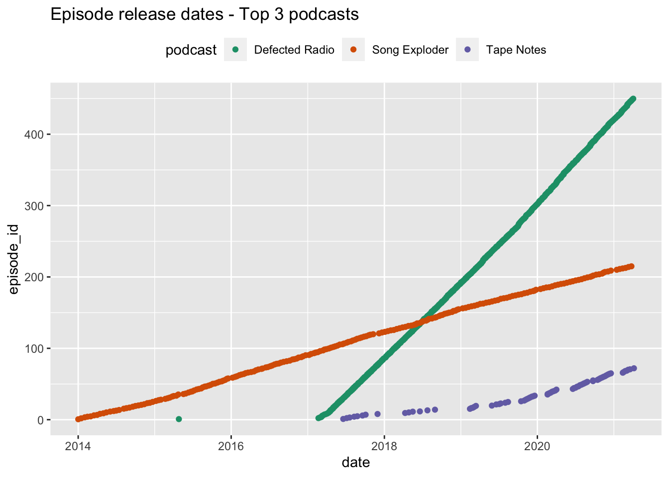
Plot Reviews for 3 podcasts
Looking at reviews for the same three podcasts, we see something strange. Although the reviews pattern for Song Exploder and Tape Notes appears to largely follow the episode timeline, the Defected Radio podcast has reviews dating back to around 2006, whereas episodes only began appearing regularly in 2015
top3 <- episode_data %>%
  filter(chart_position < 4)
top3 <- unique(top3$pod_id)
top3 <- reviews %>%
  filter(pod_id %in% top3)
top3 %>%
  ggplot() +
  aes(date, review_id, colour = podcast) +
  geom_point() +
  scale_color_brewer(palette="Dark2") +
  theme(legend.position = "top") +
  ggtitle("Review dates - Top 3 podcasts")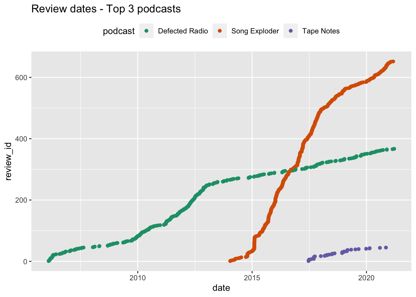
Looking at the data, this appears to be the case. Here are the date ranges for Defected Radio. We can see that the earliest episode gathered comes from 2015, while reviews go back to 2006. A likely explanation here is - just like the Joe Budden podcast above - that Defected altered or switched to a different RSS feed at some stage. Nevertheless, we have reviews covering a more recent period. However, this is an example of how basic visualisations can aid sense checking of data.
defected_episodes <- episode_data %>%
  filter(pod_id == 120107389)
range(defected_episodes$date)

defected_reviews <- reviews %>%
  filter(pod_id == 120107389)
range(defected_reviews$date)
## [1] "2015-04-26 10:00:00 UTC" "2021-04-02 08:00:00 UTC"## [1] "2006-02-08 15:10:15 GMT" "2021-03-18 11:38:27 GMT"Plot Ratings
Finally, we can briefly look at the ratings that users have given to the top 3 podcasts - shown here a percentages of the total ratings for each podcast. We can see that Tape Notes has 100% 5 star reviews, while the others have mostly 5 star reviews. Defected Radio - however - has a small percentage of negative reviews. The star rating variable may proove instructive when looking at the results of NLP analysis, which will proceed in the next section.
top3 %>%
  ggplot()+
  aes(x = podcast, fill = factor(Rating)) +
  geom_bar(position = "fill") +
  coord_flip() +
  scale_fill_brewer(palette = "Dark2") +
  theme(legend.position = "top") +
  ggtitle("Range of 1-5 Star Reviews - Top 3 podcasts")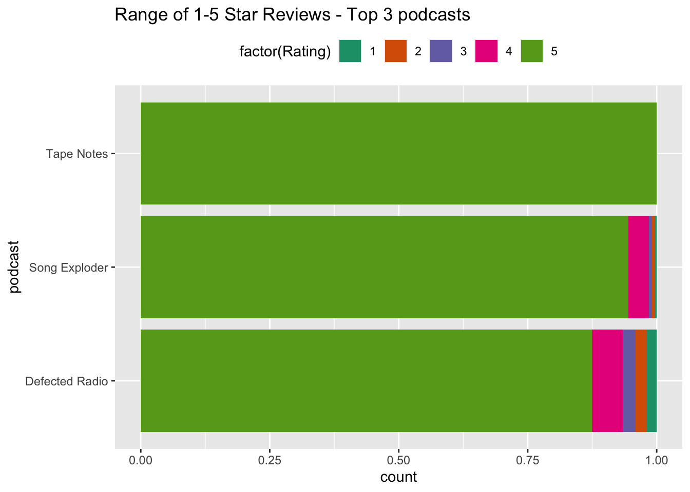
8 Save the data collected.
For the final part of this process, we can write out the four dataframes created in this part of the script so that we can return to them in Part 2.
write_rds(reviews, "reviews.rds")
write_rds(podcast_links, "podcast_links.rds")
write_rds(apple, "apple.rds")
write_rds(episode_data, "episode_data.rds")Dr Craig Hamilton
My research interests include popular music, digital humanities and online cultures.