How to get podcast ratings and reviews data using R
A tutorial - including replicable code - for using R to download all episode data and Apple reviews and ratings for a podcast.

Overview
As part of some work I’m doing at the moment with my BCMCR colleague Simon Barber, I recently set about trying out find if there was a way of getting access to the reviews and ratings posted to the Apple store about podcasts. I discovered that this information is relatively easy to get hold of, and along the way found out that getting the episode data for a podcast is also possible. Once I had the process working well, I then spent a bit of time developing it into a replicable workflow that other people could use. This post will walk you through that process.
If you are someone who makes podcasts, this should help you produce a database of your podcast episodes, an archive of listener reviews and ratings, and some quick visualisations.
In a follow up post, I will demonstrate how you can run some analysis of the data you’ve gathered and combine all elements together into a report that can be rendered as a PDF or HTML document. In this first post, however, we’ll concentrate on gathering and organising the data.
All the code required is provided below, along with explanations of what the various elements do. The code was working correctly as of 14/05/20, but please do let me know if you encounter errors. I can be contacted via email at craig.hamilton@bcu.ac.uk.
Sodajerker on Songwriting
The podcast I will be looking at in this post is Sodajerker on Songwriting. This show is made by Simon and his co-host, Brian O’Connor and - as the name suggests - it focusses on the art and craft of songwriting. Since 2011, Simon and Brian have interviewed some of the worlds most successful songwriters, including Sir Paul McCartney, Nile Rodgers, Alicia Keys, Roseanne Cash, Beck, Paul Simon, and many, many more, across 160+ episodes. It’s a great show - if you are a fan of pop music then you will almost certainly enjoy Sodajerker.
For more information on Sodajerker, visit their website or follow them on Twitter.
Ok, let’s get on with gathering the data….
1. Getting started
Load required packages
Start a new R script and load the packages below. You will also need some other packages later in the script, but I will introduce those as we go along.
library(lubridate)
library(readxl)
library(hms)
library(rvest)
library(stringr)
library(tibble)
library(dplyr)
library(tidyverse)
library(ggplot2)
Find and enter some information
To run the rest of this script you will need to find four pieces of information and assign them to specific objects in the R environment. The script below will call on these objects and use them as the basis for gathering and presenting information, so it is important that you gather and enter this information carefully. If one or more of pieces are missing or incorrect, the process will fail.
Podcast name
First, create a new object in R called podcast_name that contains the name of the podcast you will be getting data for. We’ll use this element when creating visualisations later in the script. Remember to encase the podcast name in quotation marks. Similarly, create another variable - this time with underscores - to use for writing data out.
podcast_name <- 'Name of Podcast'
podcase_file_name <- 'Name_of_podcast'
Podcast RSS feed
Next you will need the RSS feed for the podcast. This will contain all the information you need to gather episode data. You will often find the RSS link on a podcast’s website, or through one of the many podcast distribution services. You should also be able to find the RSS feed by Googling the name of the podcast + RSS feed. In the case of Sodajerker on Songwriting, their RSS feed is published on their website.
Once you have the RSS feed address, assign it to an R object called URL, again remembering to encase the address in quotation marks. Also, make sure you include the http prefix and /rss suffix - exactly as shown below.
URL <- 'https://[Podcast RSS address]/rss' Apple store ID
You will then need the ID of the podcast from the Apple store in order to retrieve the ratings and reviews. Again, this should be easy to find by Googling ‘Apple Podcast Store + Name of podcast’. You are looking for the line of digits that will appear in the URL.
Asign these digits to an object called pod_id, but do not include quotation marks.
pod_id <- #Podcast ID without quote marks, e.g. 123456789List of Apple store country codes.
Finally, you will need a list of country codes for Apple stores in different places around the world. I found what appears to be a full list here. I copied this information into an excel sheet containing two columns: code and country. The script below specifically looks for these variables.
apple <- read_excel('apple_store_codes.xlsx', sheet = 1)Once you have the object apple in your enviroment, it should look like this. The code column contains the two-character codes we will need later.
head(apple)## # A tibble: 6 × 2
## code country
## <chr> <chr>
## 1 al Albania
## 2 dz Algeria
## 3 ao Angola
## 4 ai Anguilla
## 5 ag Antigua and Barbuda
## 6 ar ArgentinaWith the information above assigned to the relevant objects in your R session, you are now ready to start collecting data. We’ll start with the episode data, and will then move on to the reviews and ratings data.
2. Get Episode Data
By following this excellent tutorial written by Robert Muwanga and using the code he supplied in his post, the following will call on the URL we created above to produce a new dataframe called episode_data
css_descriptors <- c('title', 'pubDate', 'itunes\\:summary', 'itunes\\:duration') # XML tags of interest
col_names <- c('title', 'pubdate','summary', 'duration') # Initial column names for tibble

# Load XML feed and extract items nodes
podcast_feed <- read_xml(URL)
items <- xml_nodes(podcast_feed, 'item')

# Extracts from an item node the content defined by the css_descriptor
extract_element <- function(item, css_descriptor) {
  element <- xml_node(item, css_descriptor) %>% xml_text
  element
}

episode_data <- sapply(css_descriptors, function(x) {
  extract_element(items, x)}
) %>% as_tibble()

names(episode_data) <- col_names # Set new column names
Housekeeping and tidying
Before moving on we need to perform a couple of housekeeping and tidying tasks. First we can use the lubridate package to convert the pubdata variable (the date an episode was published) into a date object
episode_data$pubdate<- dmy_hms(episode_data$pubdate) Next we need to clean up the duration variable relating to the length of each episode. This information is currently a character variable and needs to be converted with lubridate. For episodes over 60 minutes long, this is not a problem because they will appear in Hours, Minutes and Seconds (e.g a 65-minute episode will have the value 01:05:00). However, episodes that are under 60 minutes long do not have the hour data present (so, a 47-minute episode will have the value 47:00, not 00:47:00). As such the data has two different ‘shapes’ and we need to make them uniform. We can do this by splitting the data in two and adding 00: to the episodes under 60 minutes long, and then putting the data back together again. We can then use lubridate to create a new variable called duration_clean.
less_than_hour <- episode_data %>%
  filter(nchar(episode_data$duration) < 6)
more_than_hour <- episode_data %>%
  filter(nchar(episode_data$duration) > 6)
less_than_hour$duration <- paste0("00:", less_than_hour$duration)
episode_data <- rbind(less_than_hour, more_than_hour)
rm(less_than_hour, more_than_hour)
episode_data$duration_clean <- as_hms(episode_data$duration)
Then, by using the podcast_name variable we created earlier, we can add then name of the podcast to the dataframe. This will be useful if you run this script on more than one podcast and want to combine data sets later on. We can also reorder the dataframe by episode publication date, showing the earliest episode first, before then adding id numbers for each record.
#add podcast name
episode_data$podcast_name <- podcast_name

#order by date
episode_data <- episode_data[order(episode_data$pubdate , decreasing = FALSE), ]

#add ids
episode_data$id <- 1:nrow(episode_data)
In the case of Sodajerker, the resulting dataframe looks like this
str(episodes_data)## tibble [168 × 6] (S3: tbl_df/tbl/data.frame)
## $ title : chr [1:168] "Episode 1 - Billy Steinberg" "Episode 2 - Todd Rundgren" "Episode 3 - Sacha Skarbek" "Episode 4 - Jimmy Webb" ...
## $ pubdate : POSIXct[1:168], format: "2011-11-09 22:23:00" "2011-11-25 11:36:00" ...
## $ summary : chr [1:168] "In the first episode of Sodajerker On Songwriting, co-hosts Simon Barber and Brian O'Connor introduce the podca"| __truncated__ "In the second episode of Sodajerker On Songwriting, Simon and Brian talk with writer/artist/producer Todd Rundg"| __truncated__ "In the third episode of Sodajerker On Songwriting, Simon and Brian talk to Grammy nominated and two-time Ivor N"| __truncated__ "Simon and Brian talk to legendary American songwriter Jimmy Webb about the writing of classic songs like 'By Th"| __truncated__ ...
## $ duration : chr [1:168] "00:47:30" "00:25:13" "00:44:19" "00:57:44" ...
## $ duration_clean: 'hms' num [1:168] 00:47:30 00:25:13 00:44:19 00:57:44 ...
## ..- attr(*, "units")= chr "secs"
## $ podcast_name : chr [1:168] "Sodajerker On Songwriting" "Sodajerker On Songwriting" "Sodajerker On Songwriting" "Sodajerker On Songwriting" ...Basic visualisations
Using the data we’ve gathered we can now create some visualisations. For example, we can display episodes by publication date and duration of episode.
episode_data %>%
  ggplot() +
  aes(pubdate, duration_clean) +
  geom_jitter(aes(colour = "red")) +
  ggtitle(paste(podcast_name, ": Episodes - Release date and episode duration", sep = "")) +
  theme_minimal() +
  xlab("") +
  ylab("") +
  theme(legend.position="none")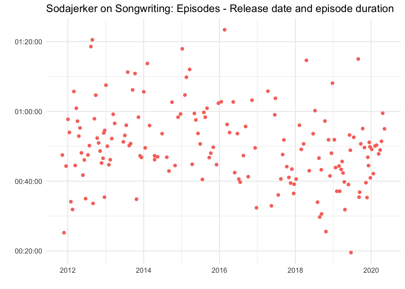
Write out the data
Before moving on to the next step - gathering Apple reviews - we can use the podcast_file_name object created earlier to write out the data in either csv or rds formats. NB:We’ll be using these rds files in the second part of the tutorial.
#Episode data
write_rds(episode_data, paste(podcast_file_name, '_episode_data.rds', sep = ""))
write.csv(episode_data, paste(podcast_file_name, '_episode_data.csv', sep = ""))
3. Get Apple ratings and reviews.
For this part of the script I used the itunesr packaged developed by amrrs. At the time of writing this package has been removed from the CRAN repository. Until it is reinstated you will need to use devtools to install it from amrrs’ Github page.
devtools::install_github("amrrs/itunesr")
library(itunesr)
The function we will use from the package is getReviews. This requires 3 inputs: the id of a podcast; the country code of the Apple store you want to get reviews and ratings from; and a page number.
We can use the pod_id variable created earlier for the first element in order to test this function out by retriving the first page of reviews for the US store. If no reviews are returned, try a different country code - ‘gb’ is the code for the UK store, for instance.
reviews <- getReviews(pod_id,'us',1) #needs ID, country and page number
reviews$country <- "us" #adds country variable
There are two unknowns as this stage. 1) which stores have reviews, and 2) if there are reviews, how many pages of reviews are there?
This was the trickiest part of the process for me to work out, but (thanks to some help from Stackoverflow!) the code below will deal with those two issues by running through the following process:
First it will iterate through each country code row in the apple dataset and check for reviews. If no reviews are returned for that country, the script will move on to the next country code, and so on until it reaches the end of the apple dataset.
If reviews are returned for a given country code they will be written to an object called reviews_test and then added to the reviews dataframe we created in the example step above.
Then, if the number of reviews returned one page 1 for a given country is 49 - the maximum number for a page - we known there is a second page of reviews. The script will then go and retrieve data from page 2 for that country.
If page 2 has fewer then 49 rows, we know that this is the last page of reviews for that country. At that point the script will break and move on to the next country code. If, however, there are 49 reviews on page 2, we know that there is a third page and the script will move on to that. This will repeat until reaching a page with fewer than 49 reviews.
Finally, and because we will by now have retrieved page 1 from the US (or GB) store twice, the last line removes duplicates from the reviews dataframe.
for (i in 1:nrow(apple)) {
  try({
    page = 1
    x <- apple$code[[i]]
    reviews_test <- getReviews(pod_id, x, page)
    reviews_test$country <- x
    reviews <- rbind(reviews, reviews_test)
    if (nrow(reviews_test) == 49)
      repeat {
        try({
          Sys.sleep(2) #This introduces a short delay and should help avoid request denial errors.
          page = page + 1
          reviews_test <- getReviews(pod_id, x , page)
          reviews_test$country <- x
          reviews <- rbind(reviews, reviews_test)
          if (nrow(reviews_test) < 49) break
        }, silent = T) #Remove , silent = T to monitor progress
      }
  }, silent = T) #Remove , silent = T to monitor progress
}

reviews <- reviews[!duplicated(reviews$Review), ]
All being well - and assuming the podcast you are looking at has been reviewed by at least one Apple user - you should now have a dataframe of reviews that looks like this.
str(reviews)## 'data.frame': 207 obs. of 8 variables:
## $ Title : chr "Well done" "Brilliant In Every Way" "Pleasing the Publishers" "Well done!" ...
## $ Author_URL : chr "https://itunes.apple.com/us/reviews/id801900430" "https://itunes.apple.com/us/reviews/id39986619" "https://itunes.apple.com/us/reviews/id139306401" "https://itunes.apple.com/us/reviews/id1083165409" ...
## $ Author_Name: chr "Orin NJ" "robert9861" "JQMusic1" "pdxpodcast" ...
## $ App_Version: chr "" "" "" "" ...
## $ Rating : num 5 5 5 5 5 5 5 5 5 5 ...
## $ Review : chr "Great interviews with great artists e.g. Tom Bailey" "I, and you, will never encounter a more brilliant podcast about the music we love, than that offered by the two"| __truncated__ "I am so grateful to you both. As an aspiring songwriter, I have soaked in every bit of information from these p"| __truncated__ "Ad free, nicely produced & well researched. A show for music lovers by music lovers!" ...
## $ Date : POSIXct, format: "2020-03-22 09:15:10" "2020-03-16 17:48:34" ...
## $ country : chr "us" "us" "us" "us" ...Visualisation
Using the reviews data we’ve just downloaded, we can then create some simple visualisaitons. For example, the chart below shows reviews by date, country and length of review.
reviews %>%
  ggplot() +
  aes(Date, nchar(Review)) +
  geom_jitter(aes(colour = country), size = 3) +
  ggtitle(paste(podcast_name, "Reviews in the Apple Store", sep = "") +
  theme_minimal() +
  xlab("") +
  ylab("Length of review") +
  theme(legend.position="top") +
  scale_color_discrete(name = "Country of Reviewer")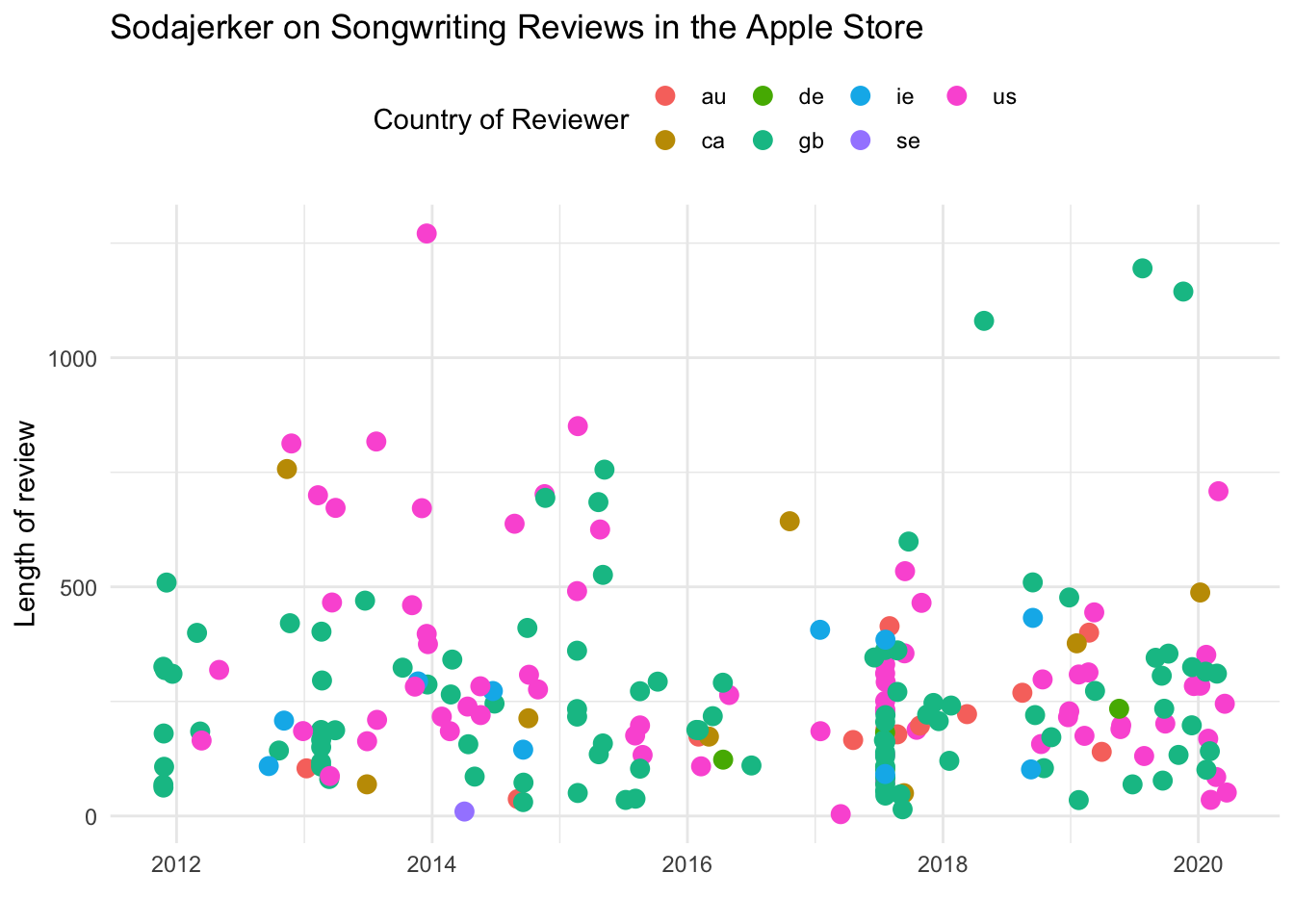
Write out reviews
Finally, you can write out the data.
write.csv(reviews, paste(podcase_file_name, "_apple_reviews.csv")
write_rds(reviews, paste(podcase_file_name, "_apple_reviews.rds")
I’ll be devling into the data we’ve gathered in a little more detail in Part 2 of this post, which I’ll be posting shortly.
In the meantime, I hope you’ve found this post useful. Please do feel free to share or use the code provided, and please also point out ways you think it could be improved (I’m sure there are several!) If you would like to talk to me about this work, or to discuss potential collaborations / other work, drop me a line or say hello on Twitter.
Dr Craig Hamilton
My research interests include popular music, digital humanities and online cultures.