The Birmingham Live Music Project Map

About BLMP

The Birmingham Live Music (BLMP) research programme examines the impact of shifts in the globalized music economy and national level changes on localised cultural, social and economic actors from the perspective of Birmingham. Its aims are to inform the public, policy-makers, and the different stakeholders involved of these effects, along with best practices and possible solutions to the different challenges faced by the globalised live music industry on a local scale.

The programme aims at a detailed mapping of the live music ecosystem in Birmingham, deploying elements of the established ‘live music census’ methodologies (replicable surveys of audiences, musicians, venues and promoters, interview and observational data, stakeholder consultation) to produce tailored qualitative and quantitative data and recommendations in the Birmingham and West Midlands context, and contribute to a broader picture of the UK’s place in the global live music economy.

‘The UK Live Music Industry in a post-2019 era: A Globalised local perspective’ is funded by the Creative Industries Policy and Evidence Centre (PEC) which is led by Nesta and funded by the Arts and Humanities Research Council.

The BLMP Map

The BLMP Birmingham Music Venue Map (v1.0) was launched on Monday 1st June 2020. You can view the map by visiting this link

The map has two main areas:

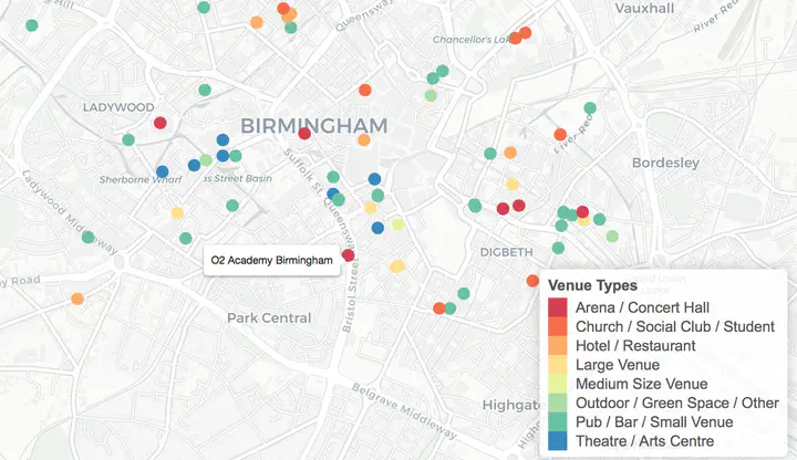
Venue Map

• An interactive map of music venues in locations with B-postcodes.
• Each venue is represented by a dot coloured by one of 8 venue types. Visitors can subset the data by one of 8 venue types by using the selection panel on the left hand side.
• By hovering over a dot the venue name will be displayed
• By clicking on a dot a venue information panel will be displayed.
• Visitors can also zoom in and out of the map, and also drag to different areas.

Venue database

• A database view of the venues on the BLMP map, organised by venue name, type, postcode, Parliamentary constituency, and ward.
• The database can be organised by any of these variables, or can be further subset using the search function.
• Visitors can subset the database by one or more of 8 venue types by using the selection panel on the left hand side.

So far, the project has gathered information for the majority of the main and major sites of live music in the city. However, and although the map currently shows 198 venues, this does not represent the full picture of live music in the city. The map therefore has a further function: a form that visitors can complete to add new venues to the database, which we hope will generate the data required to populate the map the venues we are currently missing.

Phase 1 (Feb-Mar 2020) Webscraping

An initial phase of web-scraping gathered information on Birmingham music venues from the Songkick database (see my earlier post for an overview of that process). This produced a partial list of venues and venue information, including venue names, addresses and postcodes.

The data generated in this phase was then verified and augmented by a team of 3 BLMP student assistants, who used the Songkick data as the basis for an internet search for each venue. During this phase, the research team organised venues into categories, added additional information (including social media and website links), producing a dataset of 108 venues.

Phase 2 (Mar-May 2020) Online Research

The BLMP student assistants then manually searched the internet for additional music venues not present in the Songkick database. Working through each Parliamentary constituency in the covered by a B-prefix postcode in turn, they added a further 90 venues to the database. Giving a total of 198 venues.

Based on postcode information now present in the database for each venue, the research team engaged in further web-scraping to gather supplementary data – this included information such as the nearest train station to a given venue, and the parliamentary constituency a venue was located within.

This information was combined to create the currently available version of the BLMP Map, which was created using R and deployed as a Shiny application. See this post for an overview of that process.

Phase 3 (June-August 2020) Crowdsourcing

With the launch of the BLMP Map on Monday 1st June 2020, the project entered a Crowdsourcing phase. The publicly available map contains a webform that enables local industry stakeholders and public to provide additional venue information in one of two ways:

• Venues missing from the map can be added
• Amendments to information about existing venues in the map can be suggested.

Phase 4 (July-August 2020) Verification

BLMP’s team of student assistants will monitor information submitted during the crowdsourcing phase. New venues added via the online form will be checked using internet searches and – where possible – direct contact with venue owners and managers. Likewise, suggested amendments will be verified against available information. Once additions or amendments have been verified, they will be added to the venue database.

Phase 5 (August-December 2020) Map v2.0

Based on the information gathering and verified in earlier stages, a new version of the BLMP Map will be published before December 2020

If you are new to Shiny apps

If you have never developed a Shiny application before then I would recommend this set of tutorials. They will provide you with everything you need to get started, from the basics of R programming through to app deployment.

BLMP Shiny App script

The full sample code and dataset for the Shiny app is provided below, but in this section I will break down that code into chunks to explain my decisions at certain points and to show you how you can adapt the code for your own map.

If you want to walk through the app using the sample data you can. If, however, you want to use your own data then you should structure it as follows. Ensure that all variables in your dataset are named exactly as below, and that the class of each variable matches what you see.

str(blmp_sample)

## 'data.frame':    15 obs. of  20 variables:
##  $ id              : num  67 10 93 90 22 92 23 21 46 96 ...
##  $ venue_name      : chr  "Sutton Coldfield Town Hall" "International Convention Centre" "Hamstead Social Club" "SoCa LIVE! Music Venue" ...
##  $ venue_type      : chr  "theatre" "theatre" "bar, social" "bar, smallvenue" ...
##  $ venue_add_one   : chr  "Upper Clifton Rd" "Broad Street" "311 Old Walsall Rd" "Rear of 32, Station Road" ...
##  $ venue_add_two   : chr  "Sutton Coldfield" "Birmingham" "West Bromwich East" "Yardley" ...
##  $ venue_pcode     : chr  "B736AB" "B12EA" "B421HY" "B276DN" ...
##  $ venue_web       : chr  "https://www.suttoncoldfieldtownhall.com/" "http://www.theicc.co.uk/" "http://hamsteadsocialclub.co.uk/" "https://www.socalledstudios.co.uk/soca-live" ...
##  $ venue_phone     : chr  "0121 296 9543" "0121 200 2000" "0121 357 1383" "0121 707 4152" ...
##  $ venue_email     : chr  "enquiries@townhall-scart.co.uk" "info@theicc.co.uk" "thehamsteadsocialclub@btconnect.com" "NA" ...
##  $ venue_fb        : chr  "https://en-gb.facebook.com/suttontownhall/" "https://www.facebook.com/TheICCBirmingham/" "https://www.facebook.com/pages/Hamstead-Social-Club/167225829962969" "https://www.facebook.com/socaliveuk/" ...
##  $ venue_tw        : chr  "NA" "https://twitter.com/icc_birmingham" "NA" "NA" ...
##  $ latitude        : num  52.6 52.5 52.5 52.4 52.4 ...
##  $ longitude       : num  -1.83 -1.91 -1.93 -1.82 -1.93 ...
##  $ Ward            : Factor w/ 197 levels "Abbey","Acocks Green",..: 175 104 121 2 63 32 63 132 32 32 ...
##  $ Constituency    : Factor w/ 29 levels "Aldridge-Brownhills",..: 24 6 28 10 2 6 2 8 6 6 ...
##  $ Altitude        : int  138 148 127 127 146 107 138 104 122 117 ...
##  $ Nearest.station : Factor w/ 86 levels "Acocks Green",..: 69 13 37 1 75 12 31 54 13 13 ...
##  $ ven_type_main   : chr  "Theatre" "Theatre" "Bar" "Bar" ...
##  $ train_dist_short: chr  "0.161" "0.726" "0.743" "0.233" ...
##  $ ven_type_sim    : chr  "Theatre / Arts Centre" "Theatre / Arts Centre" "Pub / Bar / Small Venue" "Pub / Bar / Small Venue" ...

First, start off your script by loading the required packages and bringing the sample dataset into the environment.

library(shiny)
library(shinydashboard)
library(tidyverse) 
library(DT)
library(leaflet) 
library(shinyWidgets)

venue_df <- read_rds('blmp_sample.rds') ## OR your dataset

Next, create two objects.

• pal will link the venue_type_sim variable to the ‘Spectral’ colour palette. We will call on this later in the script.

• all_venue_types is - as the name suggests - an ojbect containing each of the 8 unique different venue types we will plot on a map. We will also use this object in the next step, when creating an input that users can use to subset the dataset.

pal <- colorFactor(
  palette = 'Spectral',
  domain = venue_df$ven_type_sim
)  ### For adding colour to dots

all_venue_types <- sort(unique(venue_df$ven_type_sim))

The next element creates the sidebar of the dashboard.

• The pickerInput element will create a drop down menu based on everything inside all_venue_types.
• The various menuItems will create links to other areas of the app that are created in the next step.
• The tabname element within each dictates the content this link will take users to.

header <- dashboardHeader(
  title= "BLMP Map"
)

sidebar <- dashboardSidebar(
  
  sidebarMenu(
    
    pickerInput("venue_type","Select Venue Type(s):", 
                choices= c("Theatre / Arts Centre", "Pub / Bar / Small Venue", "Outdoor / Green Space / Other", 
                           "Medium Size Venue","Large Venue", "Hotel / Restaurant", 
                           "Church / Social Club / Student", "Arena / Concert Hall"), 
                options = list(`actions-box` = TRUE),
                selected = all_venue_types,
                multiple = T),
    
    menuItem("Venue Map", icon = icon("None"),
             tabName = "dashboard"
    ),
    
    menuItem("Venue Database", icon = icon("None"),
             tabName = "venue_dbase"
    ),
    menuItem("Add/Amend a Venue", icon = icon("None"),
             tabName = "add_venue"
    ),
    menuItem("About BLMP", icon = icon("None"),
             tabName = "about_project"
    ),
    menuItem("External Links", icon = icon("None"),
             
             menuSubItem(text= "Website", href = "https://[YOUR WEBSITE]"),
             menuSubItem(text= "Twitter", href = "https://YOUR TWITTER"),
             menuSubItem(text= "Facebook", href = "https://[YOUR FB]")
    )
  )
)

The body of the dashboard (everything in the main panel to the right of the sidebar) is then populated with various dynamic elements, or else static information.

• The venue_map sits in the main dashboard tab.
• The venue_dbase tab will eventually be populated with an output called venuetable, which will created on the server side.
• The about_project tab is populated with static text - in other words, this page will not change (unless you want it to an asign a dynamic element to it.
• The add_venue tab will eventually be populated by an htmlOutput that will render an online form. We’ll discuss that in a few steps.

body <- dashboardBody( 
  tabItems(
    tabItem("dashboard",
            fluidRow( 
              box(width = "12"
                  ,leafletOutput("venue_map", height = "600px")
              )
            ) 
    ),
    tabItem("venue_dbase",
            h3("Venue Database"),
            p("Some text about the database"),
            p(), DT::dataTableOutput(outputId = "venuetable")
    ),

    tabItem("about_project",
            h2("About Your Project"),
            p("Some text about your project")
    ),
    tabItem("add_venue",
            p(), htmlOutput("survey")
    )
  )
)

Finally, you complete the UI side by giving your app a title, and making selections based on other arguments, such as the skin colour.

#completing the ui part with dashboardPage
ui <- dashboardPage(title = 'Your Title', header, sidebar, body, skin= "red")

On the server side, the first task is to create a reactive dataframe that will change as users add or remove venue types from the pickerInput we have created on the UI side. This will create a ‘new’ version of the database each time the choices of venue type changes.

# create the server functions for the dashboard  
server <- function(input, output) {
  
  # Create reactive data frame   
  venue_sample <- reactive({
    req(input$venue_type)
    venue_sample <- venue_df %>%
      filter(ven_type_sim %in% input$venue_type)
    
  })    

We then need to create the venue_map object that will sit on the UI-side dashboard.

• First, we look for the latest version of venue_sample.
• Next, we create an object called content that will contain information about each venue that will appear in pop-up windows.
• Then we populate the map with latitude and longitude data, and use the content object to provide additional data.

  output$venue_map <- renderLeaflet({
    venue_sample <- venue_sample()
    content <- paste("<h3>", venue_sample$venue_name, "</h3>",
                     "<b>", "Address:", "</b>", venue_sample$venue_add_one, venue_sample$venue_add_two, venue_sample$venue_city, "<br>",
                     "<b>", "Postcode: ", "</b>", venue_sample$venue_pcode, "<br>",
                     "<b>", "Links:", "</b>","<a href='", venue_sample$venue_web,"'", "target='_blank'>", "Website", "</a>", " / ", 
                     "<a href='", venue_sample$venue_fb, "'", "target='_blank'>", "Facebook", "</a>", " / ",
                     "<a href='", venue_sample$venue_tw, "'", "target='_blank'>", "Twitter", "</a>", "<br>",
                     "<b>", "Phone: ", "</b>", venue_sample$venue_phone, "<br>",
                     "<b>", "Venue Type: ", "</b>", venue_sample$ven_type_sim, "<br>",
                     "<b>", "Nearest Train Station: ", "</b>", venue_sample$Nearest.station, "<br>",
                     "<b>", "Distance to nearest train station:", "</b>", venue_sample$train_dist_short, " miles", "<br>",
                     "<b>", "Parl. Constituency:", "</b>", venue_sample$Constituency, "<br>",
                     "<b>", "Altitude:", "</b>", venue_sample$Altitude, " metres", "<br>"
                     
                     
    )
    leaflet(venue_sample) %>%
      setView(lng = -1.8990, lat = 52.4778, zoom = 14) %>%
      addProviderTiles(providers$CartoDB.Positron) %>% 
      addCircleMarkers(~longitude, ~latitude, popup = ~content, 
                       label = ~venue_name, 
                       color = ~pal(ven_type_sim),
                       stroke = FALSE, fillOpacity = 1,
                       radius = 6) %>%
      addLegend("bottomright", pal = pal, values = ~ven_type_sim,
                title = "Venue Types",
                labFormat = labelFormat(prefix = ""),
                opacity = 1)
  })

Likewise, the venuetable output first looks for the latest version of venue_sample, then - after selected the coloumns we need - creates a datatable

  output$venuetable <- DT::renderDataTable({
    venue_sample <- venue_sample()
    DT::datatable(data = venue_sample[,c(2:3, 6, 18:19)], 
                  options = list(pageLength = 10),
                  rownames = FALSE,
                  colnames = c("Venue Name", "Venue Type", "Postcode", "Constituency", "Ward"))
  })
}

Then, we can embed an online survey in an iframe object that will be rendered on the add a venue tab created on the UI side.

  output$survey <- renderUI({
    tags$iframe(width= "100%", height = "1800", src ="[THE EMBED CODE OF A FORM OR SURVEY]", frameborder="0", marginheight="0", marginwidth="0")
  })

Finally, the script ends by pulling together the UI and server elements into a shinyApp.`

shinyApp(ui = ui, server = server)

Sample code and Shiny script

The full code required to run create an application similar to the one I produced for the BLMP project is available here. This code was working as of 26/05/20 and – along with the sample dataset I’ve provided – should work in your local installation of R Studio.

Publishing your app

If you adapt the code for your own use and want to make it available online you have two options. The easy way is to publish your app to shinyapps.io from R Studio. This will produce a working version of your app that you can share with others. Shinyapps offers a free tier based on limited use that may be sufficient for your needs. If, however, you anticipate a decent amount of use on your app then you would have to explore the paid tiers, which begin at US$9 per month. Visit Shinyapps.io for more information on that.

If you want something a little more longer-term and/or with a greater use capacity, you may want to investigate creating your own Shiny server on which to host your new app, and any subsequent ones you build. I discuss how you might go about that in the next section.

Tutorial 2, Step 9.2

In this part, ensure that you install ALL the packages required by your Shiny server app. Saskia’s tutorial shows you how to install R packages for all users on your server, but the mistake I made in following this was to only install the packages shown in the tutorial. This was a silly error, but it resulting in my app failing later on - because the packages required to run it were not installed.

(Another note here: installing all the packages required takes quite some time; around 40 minutes in the case of the BLMP app)

Tutorial 2, Step 12

Despite following Saskia’s instructions I was unable to make my server appear on my domain name correctly, and my app did not work on an https connection. In trying to troubleshoot this problem I came across this resource from Digital Ocean. After running through this process instead, my app became visible on my domain through both http and https connections. My advice here would be to follow Saskia’s tutorial first, and then use the alternate method is a fallback if you encounter problems.